Thresholds
Thresholds are the simplest type of filter in latools. They identify regions where the concentration or local gradient of an analyte is above or below a threshold value.
Appropriate thresholds may be determined from prior knowledge of the samples, or by examining whole-analysis level cross-plots of the concentration or local gradients of all pairs of analytes, which reveal relationships within all the ablations, allowing distinct contaminant compositions to be identified and removed.
Tip
All the following examples will work on the example dataset worked through in the Beginner’s Guide. If you try multiple examples, be sure to run eg.filter_clear() in between each example, or the filters might not behave as expected.
Concentration Filter
Selects data where a target analyte is above or below a specified threshold.
For example, applying an threshold Al/Ca value of 100 μmol/mol to Sample-1 of the example data:
# Create the filter.
eg.filter_threshold(analyte='Al27', threshold=100e-6)
This creates two filters - one that selects data above the threshold, and one that selects data below the threshold. To see what filters you’ve created, and whether they’re ‘on’ or ‘off’, use filter_status(), which will print:
Subset All_Samples:

n  Filter Name          Mg24   Mg25   Al27   Ca43   Ca44   Mn55   Sr88   Ba137  Ba138
0  Al27_thresh_below    False  False  False  False  False  False  False  False  False
1  Al27_thresh_above    False  False  False  False  False  False  False  False  False
To effect the data, a filter must be activated:
# Select data below the threshold
eg.filter_on('Al27_below')

# Plot the data for Sample-1 only
eg.data['Sample-1'].tplot(filt=True)
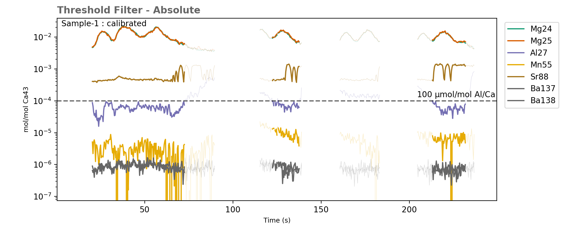
Data above the threshold values (dashed line) are excluded by this filter (greyed out).
Tip
When using filter_on() or filter_off(), you don’t need to specify the entire filter name displayed by filter_status(). These functions identify the filter with the name most similar to the text you entered, and activate/deactivate it.
Gradient Filter
Selects data where a target analyte is not changing - i.e. its gradient is constant. This filter starts by calculating the local gradient of the target analyte:
Calculating a moving gradient for the Al27 analyte. When calculating the gradient the win parameter specifies how many points are used when calculating the local gradient.
For example, imagine a calcium carbonate sample which we know should have constant Al concentration. In this sample, variable Al is indicative of a contaminant phase. A gradient threshold filter can be used to isolate regions where Al is constant, and more likeley to be contaminant-free. To create an apply this filter:
eg.filter_gradient_threshold(analyte='Al27', threshold=0.5e-5, win=25)

eg.filter_on('Al27_g_below')

# plot the gradient for Sample-1
eg.data['Sample-1'].gplot('Al27', win=25)
# plot the effect of the filter for Sample-1
eg.data['Sample-1'].tplot(filt=True)
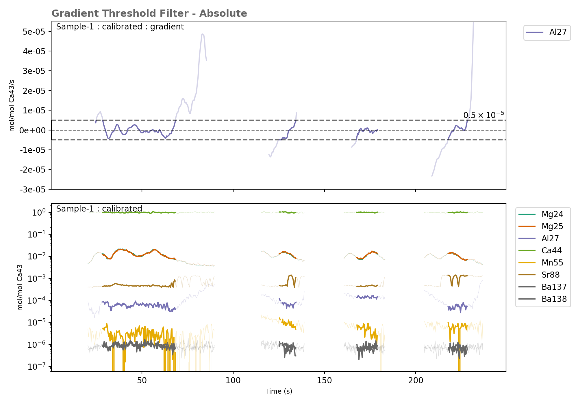
The top panel shows the calculated gradient, with the regions above and below the threshold value greyed out. the bottom panel shows the data regions selected by the filter for all elements.
Choosing a gradient threshold value
Gradients are in units of mol[X] / mol[internal standard] / s. The absolute value of the gradient will change depending on the value of win used.
Working out what a gradient threshold value should be from first principles can be a little complex.
The best way to choose a threshold value is by looking at the data.
There are three functions to help you do this:
gradient_plots()Calculates the local gradient of all samples, plots the gradients, and saves them as a pdf. The gradient equivalent oftrace_plots().gradient_histogram()Plot histograms of the local gradients in the entire dataset.gradient_crossplot()Create crossplots of the local gradients for all analyes.
Tip
The value of win used when calculating the gradient will effect the absolute value of the calculated gradient. Make sure you use the same win value creating filters and viewing gradients.
Related Functions
filter_threshold()creates a threshold filter.filter_on()andfilter_off()turn filters on or off.gradient_plots()Calculates the local gradient of all samples, plots the gradients, and saves them as a pdf. The gradient equivalent oftrace_plots().gradient_crossplot()Create crossplots of the local gradients for all analyes.gradient_histogram()Plot histograms of the local gradients in the entire dataset.trace_plots()with optionfilt=Truecreates plots of all data, showing which regions are selected/rejected by the active filters.filter_reports()creates plots of a particular filter, showing which sections of the ablation are selected.filter_clear()deletes all filters.
Percentile Thresholds
In cases where the absolute threshold value is not known, a percentile may be used. An absolute threshold value is then calculated from the raw data at either the individual-ablation or population level, and used to create a threshold filter.
Warning
In general, we discourage the use of percentile filters. It is always better to examine and understand the patterns in your data, and choose absolute thresholds. However, we have come across cases where they have proved useful, so they remain an available option.
Concentration Filter: Percentile
For example, to remove regions containing the top 10% of Al concentrations:
eg.filter_threshold_percentile(analyte='Al27', percentiles=90)

eg.filter_on('Al_below')

eg.data['Sample-1'].tplot(filt=True)
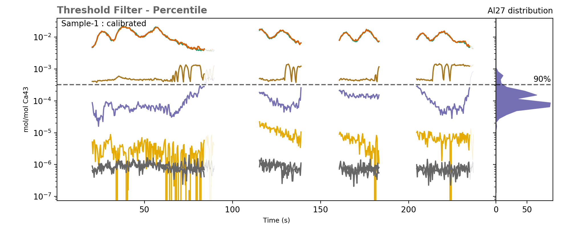
The histogram on the right shows the distribution of Al data in the sample, with a line showing the 90th percentile of the data, corresponding to the threshold value used.
Gradient Filter: Percentile
The principle of this filter is the same, but it operatures on the local gradient of the data, instead of the absolute concentrations.