Long File Splitting
If you’ve collected data from ablations of multiple samples and standards in a single, long data file, read on.
To work with this data, you have to split it up into numerous shorter files, each containing ablations of a single sample.
This can be done using latools.preprocessing.split.long_file().
Ingredients
- A single data file containing multiple analyses
- A Data Format description for that file (you can also use pre-configured formats).
- A list of names for each ablation in the file.
To keep things organise, we suggest creating a file structure like this:
my_analysis/
    my_long_data_file.csv
    sample_list.txt
Tip
In this example we’ve shown the sample list as a text file. It can be in any format you want, as long as you can import it into python and turn it into a list or array to give it to the splitter function.
Method
- Import your data, and provide a list of sample names.
- Apply
autorange()to identify ablations.- Match the sample names up to the ablations.
- Save a single file for each sample in an output folder, which can be imported by
analyse()- Plot a graph showing how the file has been split, so you can make sure everything has worked as expected.
Output
After you’ve applied long_file(), a few more files will have been created, and your directory structure will look like this:
my_analysis/
    my_long_data_file.csv
    sample_list.txt
    my_long_data_file_split/
        STD_1.csv
        STD_2.csv
        Sample_1.csv
        Sample_2.csv
        Sample_3.csv
        ... etc.
If you have multiple consecutive ablations with the same name (i.e. repeat ablations of the same sample) these will be saved to a single file that contains all the ablations of the same file.
Example
To try this example at home this zip file contains all the files you’ll need.
Unzip this file, and you should see the following files:
long_example/
    long_data_file.csv  # the data file
    long_data_file_format.json  # the format of that file
    long_example.ipynb  # a Jupyter notebook containing this example
    sample_list.txt  # a list of samples in plain text format
    sample_list.xslx  # a list of samples in an Excel file.
1. Load Sample List
First, read in the list of samples in the file. We have examples in two formats here - both plain text and in an Excel file. We don’t care what format the sample list is in, as long as you can read it in to Python as an array or a list. In the case of these examples:
Text File
import numpy as np
sample_list = np.genfromtxt('long_example/sample_list.txt',  # read this file
                            dtype=str,  # the data are in text ('string') format
                            delimiter='\n',  # separated by new-line characters
                            comments='#'  # and lines starting with # should be ignored.
                            )
This loads the sample list into a numpy array, which looks like this:
array(['NIST 612', 'NIST 612', 'NIST 610', 'jcp', 'jct', 'jct',
       'Sample_1', 'Sample_1', 'Sample_1', 'Sample_1', 'Sample_1',
       'Sample_2', 'Sample_2', 'Sample_2', 'Sample_3', 'Sample_3',
       'Sample_3', 'Sample_4', 'Sample_4', 'Sample_4', 'Sample_5',
       'Sample_5', 'Sample_5', 'Sample_5', 'Sample_5', 'Sample_5',
       'NIST 612', 'NIST 612', 'NIST 610', 'jcp', 'jct', 'jct'],
      dtype='<U8')
Excel File
import pandas as pd
sample_list = pd.read_excel('long_example/sample_list.xlsx')
This will load the data into a DataFrame, which looks like this:
| Order | Samples |
|---|---|
| 1 | NIST 612 |
| 2 | NIST 612 |
| 3 | NIST 610 |
| 4 | jcp |
| 5 | jct |
| 6 | jct |
| 7 | Sample_1 |
| 8 | Sample_1 |
| 9 | Sample_1 |
| 10 | Sample_1 |
| 11 | Sample_1 |
| 12 | Sample_2 |
| 13 | Sample_2 |
| 14 | Sample_2 |
| 15 | Sample_3 |
| 16 | Sample_3 |
| 17 | Sample_3 |
| 18 | Sample_4 |
| 19 | Sample_4 |
| 20 | Sample_4 |
| 21 | Sample_5 |
| 22 | Sample_5 |
| 23 | Sample_5 |
| 24 | Sample_5 |
| 25 | Sample_5 |
| 26 | Sample_5 |
| 27 | NIST 612 |
| 28 | NIST 612 |
| 29 | NIST 610 |
| 30 | jcp |
| 31 | jct |
| 32 | jct |
The sample names can be accessed using:
sample_list.loc[:, 'Samples']
2. Split the Long File
import latools as la

fig, ax = la.preprocessing.long_file('long_example/long_data_file.csv',
                                     dataformat='long_example/long_data_file_format.json',
                                     sample_list=sample_list.loc[:, 'Samples'])  # note we're using the excel file here.
This will produce some output telling you what it’s done:
The single long file has been split into 13 component files in the format that latools expects - each file contains ablations of a single sample.
Note that consecutive ablations with the same sample are combined into single files, and if a sample name is repeated _N is appended to the sample name, to make the file name unique.
The function also produces a plot showing how it has split the files:

3. Check Output
So far so good, right? NO! This split has not worked properly.
Take a look at the printed output. On the second line, it says that the number of samples in the list and the number of ablations don’t match. This is a red flag - either your sample list is wrong, or latools is not correctly identifying the number of ablations.
The key to diagnosing these problems lies in the plot showing how the file has split the data. Take a look at the right hand side of this plot:
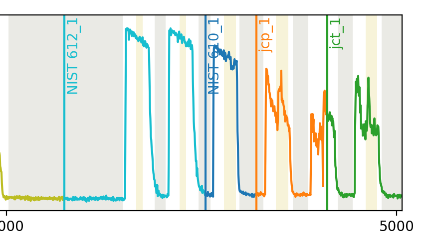
Something has gone wrong with the separation of the jcp and jct ablations.
This is most likely related to the signal decreasing to close to zero mid-way through the the second-to-last ablation, causing it to be itendified as two separate ablations.
4. Troubleshooting
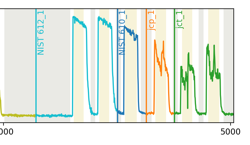
In this case, a simple solution could be to smooth the data before splitting.
The long_file() function uses autorange() to identify ablations in a file, and you can modify any of the autorange parameters by passing giving them directly to long_file().
Take a look at the autorange() documentation. Notice how the input parameter swin applies a smoothing window to the data before the signal is processed. So, to smooth the data before splitting it, we can simply add an swin argument to long_file():
fig, ax = la.preprocessing.long_file('long_example/long_data_file.csv',
                                     dataformat='long_example/long_data_file_format.json',
                                     sample_list=sample_list.loc[:, 'Samples'],
                                     swin=10)  # I'm using 10 here because it seems to work well... Pick whatever value works for you.
This produces the output:
You can see in the image that this has fixed the issue:
5. Analyse
You can now continue with you latools analysis, as normal.
dat = la.analyse('long_atom/10454_TRA_Data_split', config='REPRODUCE', srm_identifier='NIST')
dat.despike()
dat.autorange(off_mult=[1, 4.5])
dat.bkg_calc_weightedmean(weight_fwhm=1200)
dat.bkg_plot()
dat.bkg_subtract()
dat.ratio()
dat.calibrate(srms_used=['NIST610', 'NIST612'])
_ = dat.calibration_plot()

# and etc...